Other Compartmental Models
The SEIR Model
The SEIR model is a simple extension of the basic SIR model to include the Exposed state to account for disease pathologies that go through a latent phase where an individual hasn’t started infecting others despite being exposed to the disease. The Exposed compartment (E) represents this incubation period for the disease. The infected individuals expose the Susceptible individuals (S) to the disease, moving the latter into the Exposed (E) compartment before they are moved to the Infected (I) compartment. From the infected compartment they will be Removed (R) eventually. Here we use the “Removed” compartment to indicate that individuals are removed from contributing to the disease spread. This could mean permanently recovered, immune, or dead. The diagram below shows how the individuals move through each compartment in this model.
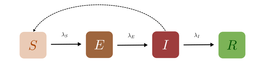
The rate at which the disease is transmitted from an infected agent to a susceptible agent is represented by \({\lambda_S}\) (transmission rate). The incubation rate, \({\lambda_E}\), is the rate of Exposed individuals becoming infectious. The average time an individual spends in the Exposed compartment is given by \({1/\lambda_E}\). Lastly, \({\lambda_I}\) represents the rate of removal of infected individuals from the Infected compartment.
In a closed population with no births or deaths, the SEIR model can be defined using a set of coupled non-linear differential equations described below:
where the total population,
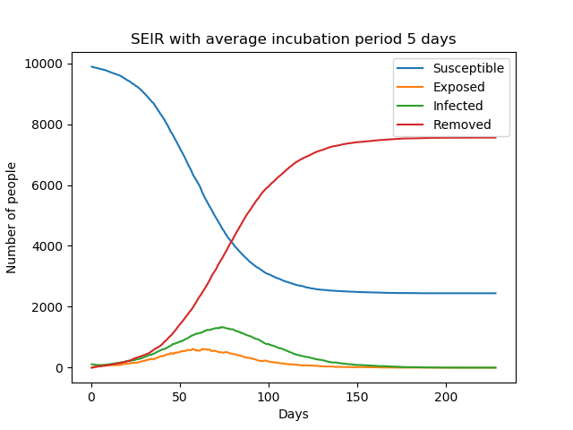
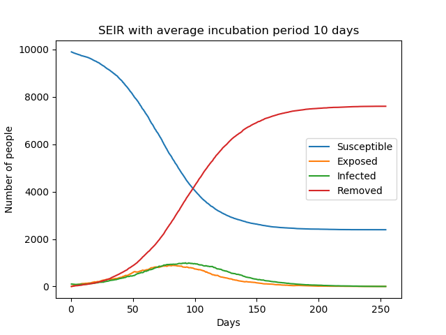
Introducing the incubation period does not change the total number of infections, but prolongs the duration of the epidemic. The graphs below show simple SEIR models with incubation periods 5 and 10 days respectively.
The above equations can be solved numerically to get deterministic results but, as explained in The SIR Model, we can also solve it stochastically using a similar algorithm.
In the algorithm, if the agent is Susceptible, we compute the number of infected individuals they come in contact with who could potentially infect them (\(I\)). Then, during each time step \({\Delta t}\), they are transferred to the Exposed compartment, with some probability,
Individuals from the Exposed compartment are transferred to the Infected compartment with the probability,
If the agent is already infected, we transition them to the Removed compartment with a probability
Similarly to the SIR model, the average of the stochastic solutions come close to the mean field solution, as seen in the figure below.
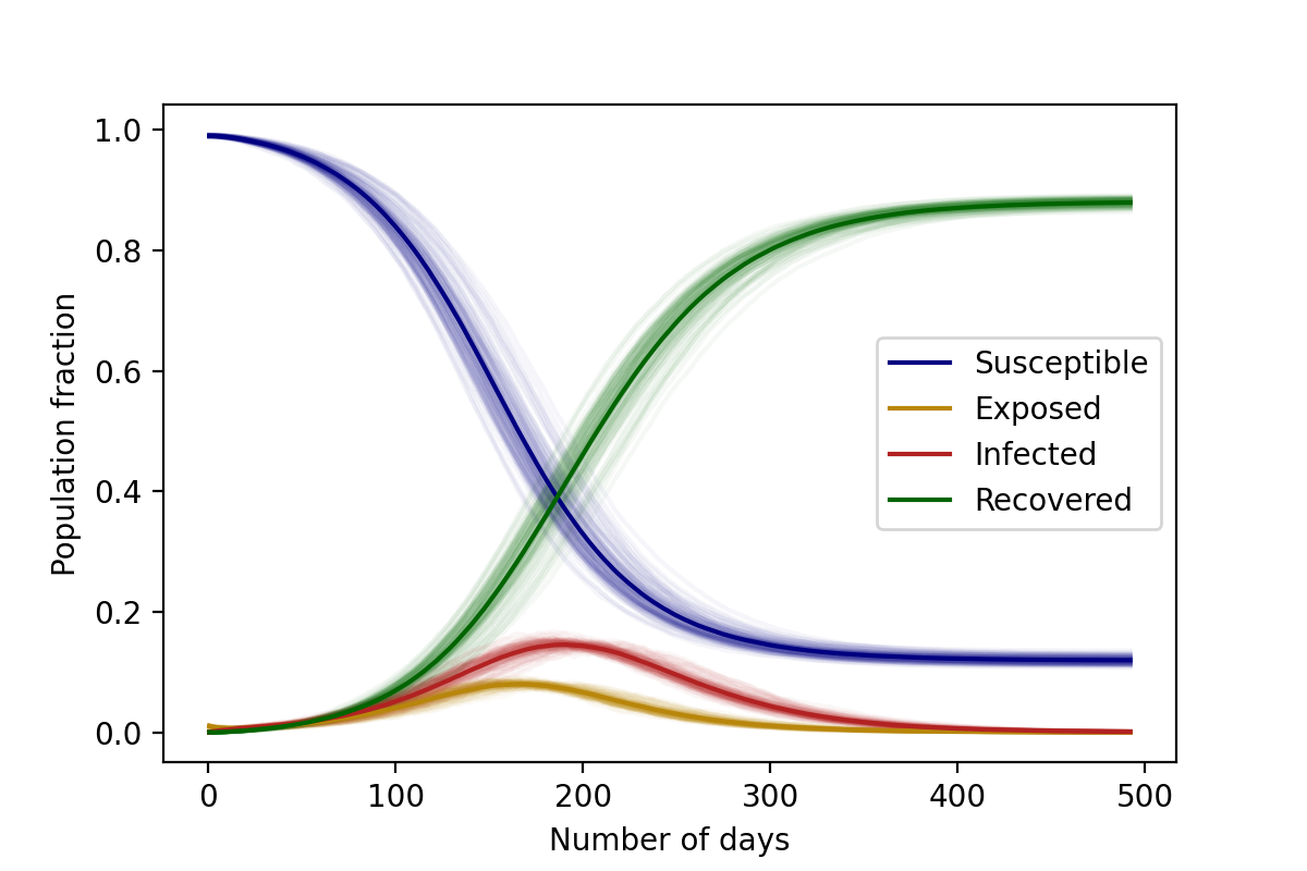
\(\lambda_S=3/35 \text{ day}^{-1}\), \(\lambda_E=1/14 \text{ day}^{-1}\), \(\lambda_I=1/28 \text{ day}^{-1}\), \(N=10,000\).
Initial conditions: 1% Infected, 99% Susceptible
The SAIR Model
In the models we have described so far, we have not distinguished between the types of infected individuals in the population. In many real-world situations, however, we might need to make this distinction. For example, the disease progression of mildly infected individuals might be very different from severely infected individuals. Additionally, the existence of asymptomatic individuals may be crucial in studying the efficiency of non-pharmaceutical interventions such as quarantining individuals.
Let us begin by examining a very basic case: a generalisation of the The SIR Model to include both symptomatic (\(I\)) and asymptomatic (\(A\)) individuals. Such a distinction might be important to study the spread of epidemics like COVID-19, especially because asymptomatic individuals are much more likely to spread the disease as they are hard to indentify without extensive testing and contact tracing. From these compartments the individuals move to the Removed (\(R\)) compartment, at rates \(\lambda_A\) and \(\lambda_I\) respectively, as shown in the disease progression below.
In the models described so far, we have assumed that all infections are equal in their severity or intensity. However, in many real-world diseases, the disease manifests itself differently across individuals. For example, some individuals might be mildly infected, some might mount a severe symptomatic response, while others might be entirely asymptomatic. Accounting for these different types of infections is crucial to accurately model the disease progression through the population. Let us begin by examining a very basic case: a generalisation of the The SIR Model to include both symptomatic (\(I\)) and asymptomatic (\(A\)) individuals. Such a distinction might be important to study the spread of epidemics like COVID-19 and guide understanding and interventions. For instance, asymptomatic individuals might end up spreading the disease far and wide since they are hard to identify without extensive testing and contact tracing. Similarly, if we can predict the trajectory of severe cases, healthcare measures can be taken appropriately. From both these compartments the individuals move to the Removed (\(R\)) compartment, at rates \(\lambda_A\) and \(\lambda_I\) respectively, as shown in the disease progression below.
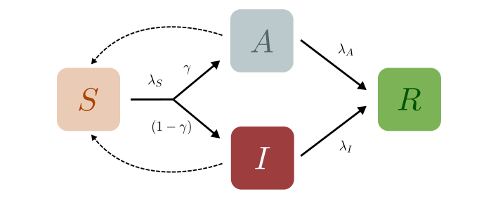
Initially, we can assume that both asymptomatic and symptomatic individuals infect susceptibles with equal capacity. (In reality, this capacity depends on various nuanced aspects of the disease pathology and the network of interacting individuals. However, we won’t delve into those details here.) We call this transition rate out of \(S\), \(\lambda_S\), as before.
However, now a branching event can occur. Once infected, a susceptible person could either move to \(A\) or \(I\). We thus define another quantity, \(\gamma\), which is the fraction of the infected individuals who are asymptomatic. The individuals then transit out of \(A\) or \(I\) with rates \(\lambda_A\) or \(\lambda_I\) respectively. The set of coupled non-linear differential equations that defines the SAIR model in a closed population are:
where, just as before, the total population is constant:
Exercise
Convince yourself that if \(\lambda_A = \lambda_I\), this model effectively reduces to a simple \(SIR\) model. In this case the distinction between the asymptomatics and symptomatics is merely cosmetic.
Modelling the transitions in the SAIR model is a little bit more involved than in the SIR model, though the basic principle is the same.
Warning
One might naively imagine that we could simply write:
and draw two random numbers \(r_1\) and \(r_2\) to check if \(P_\text{SA}\) or \(P_\text{SI}\) occur. However, this is not strictly correct. The transitions from \(S\) to \(A\) and from \(S\) to \(I\) are not independent transitions, and therefore you cannot simply treat them like we have in the previous models. However, there are two independent transitions: the transition out of \(S\), and the branching to \(A\) or \(I\).
Thus, at each tick \(\Delta t\), susceptible individuals are checked for infection and are moved out of the susceptible compartment with a probability
Now, once they are set to transition, they are either sent to \(A\) with a probability \(\gamma\), or otherwise they are sent to \(I\). The asymptomatic and symptomatic individuals are finally transferred to the Removed compartment with a probabilities \(\lambda_A\Delta t\) and \(\lambda_I\Delta t\) respectively.
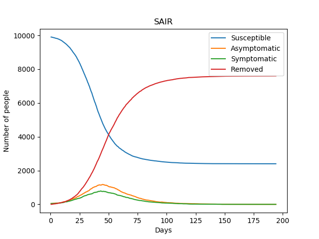
Once again, we can see the differential equation solutions as the average of the stochastic ones, as demonstrated in the figure below.
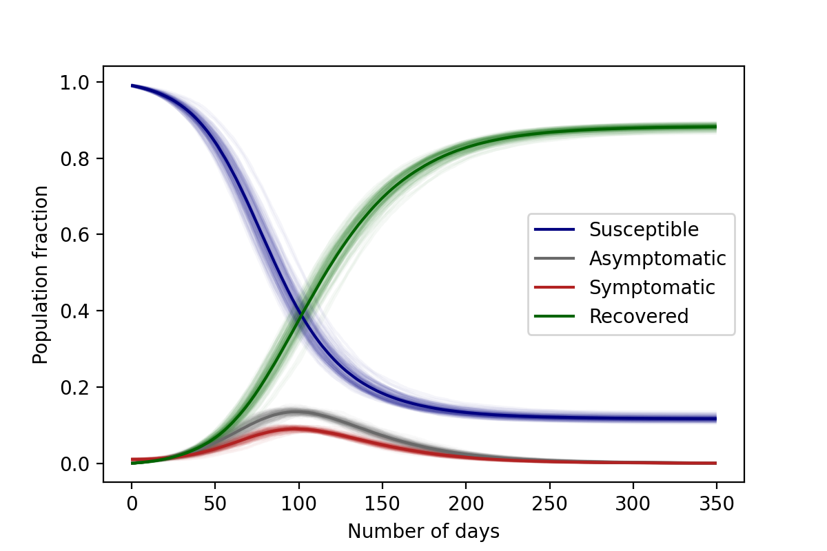
\(\lambda_S=3/35 \text{ day}^{-1}\) , \(\lambda_A=1/28 \text{ day}^{-1}\), \(\lambda_I=1/28 \text{ day}^{-1}\), \(\gamma=0.6\), \(N=10,000\)
Initial conditions: 1% Asymptomatic, 99% Susceptible
We can now add one last level of complexity to this problem: what if we wanted to model a situation in which asymptomatic individuals are less likely to infect susceptibles (perhaps because they have a lower viral load) than symptomatics. In this case, we would like to include a sort of “relative risk” of infection from an asymptomatic individual that is smaller than the risk of being infected by a symptomatic individual. In order to do this, we can introduce some “contact parameters” that modulate the \(S\to A\) and \(S\to I\) transitions. In this case the differential equations can be written as:
Thus, if \(C_I = 1\) and \(C_A = 0.5\), then a single asymptomatic individual is only half as likely as a symptomatic individual at infecting a susceptible person.
Note
Notice how the quantities that really matter re not \(C_A\) or \(C_I\), but rather \(\lambda_S\, C_A\) and \(\lambda_S\, C_I\). If you were to choose \(C_I = 2\) and \(C_A = 1\), in this case as well asymptomatics will be half as likely like to infect susceptibles, but we have effectively increased the overall value of \(\lambda_S\) because of the factor 2.
Exercise
In this case, would setting \(\lambda_A = \lambda_I\) reduce this to a simple SIR model, as before? Why not?
The SIRS Model
In the SIR model, recovered individuals attain life long immunity. However, this is not the case for many diseases. The acquired immunity can decline over time and as a result the recovered individuals can get reinfected. The SIRS (Susceptible – Infected – Recovered – Susceptible) model allows us to transfer recovered individuals back to the Susceptible compartment. The diagram below shows the movement of the individuals through each compartment in an SIRS model.
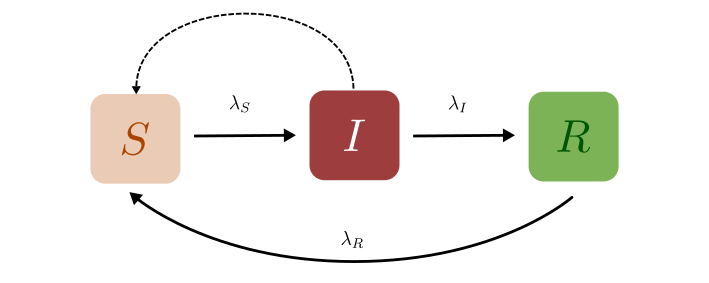
The infectious rate, \(\lambda_S\), represents the probability of transmitting disease between a susceptible and an infectious individual. \(\lambda_I\) is the recovery rate which can be determined from the average duration of infection.
\(\lambda_R\) is the rate at which the recovered individuals return to the susceptible statue due to loss of immunity.
Ignoring the vital dynamics (births and deaths), in the deterministic form, the SIRS model can be written as the following ordinary differential equations:
where the total population is,
The main difference between this model and the SIR model is now that because of the possibility of reinfections, there also exists the possibility of multiple _waves_ of infection. In the example below, we can see the emergence of a second wave (easily visible by seeing an increase in \(R(t)\) from days 150-200):
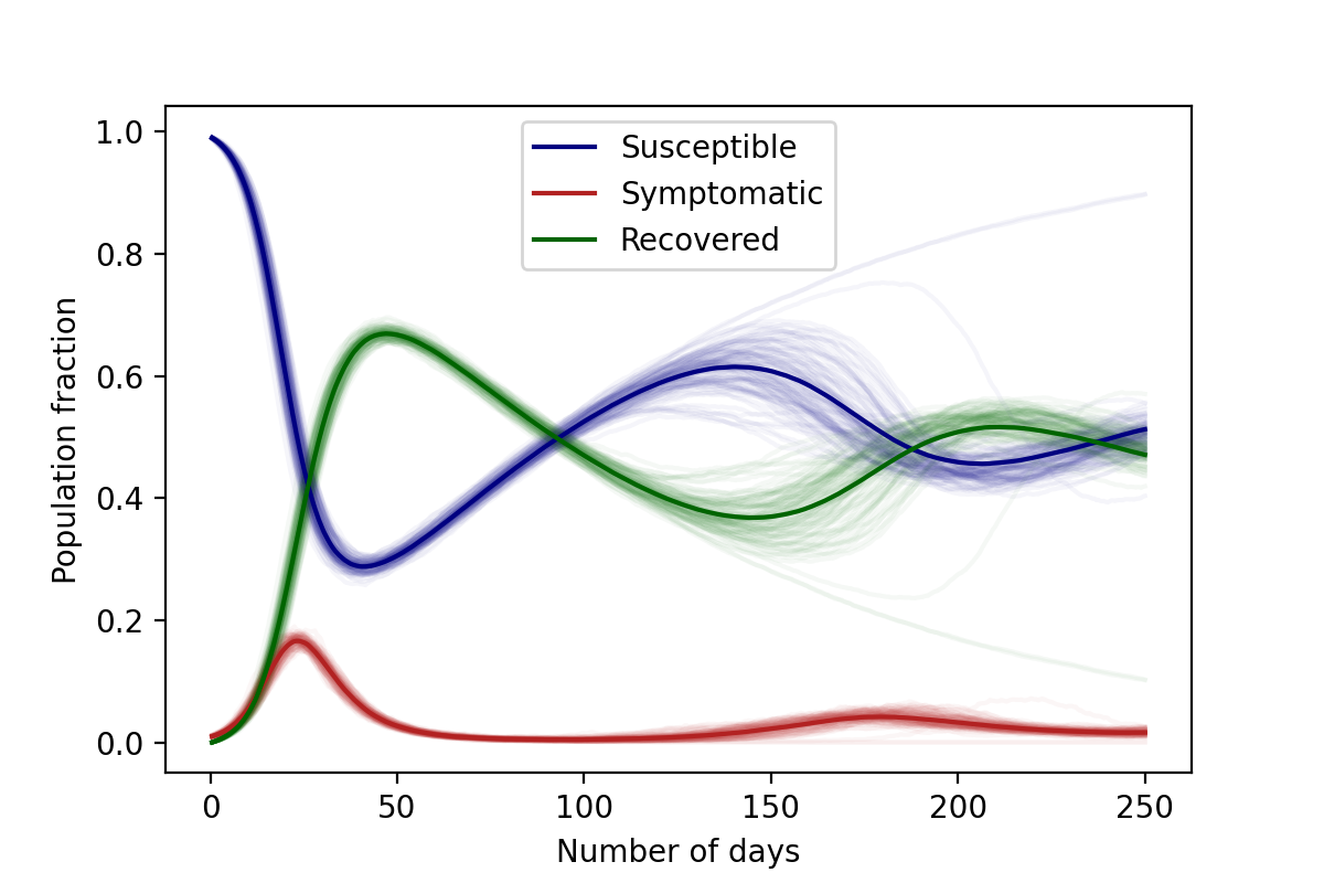
Parameters: \(\lambda_S=2/5 \text{ (day)}^{-1}\), \(\lambda_I=1/5 \text{ (day)}^{-1}\), \(\lambda_R=1/100 \text{ (day)}^{-1}\), \(N=10,000\).
Initial conditions: 1% Infected, 99% Susceptible
On choosing the right parameters, an endemic equilibrium can be reached, meaning that the disease never truly dies out: some small fraction of the population is always infected, as shown below.
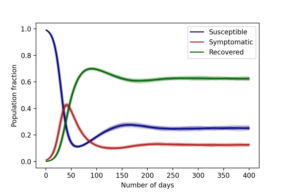
Parameters: \(\lambda_S=1/5 \text{ day}^{-1}\), \(\lambda_I=1/20 \text{ day}^{-1}\), \(\lambda_R=1/100 \text{ day}^{-1}\), \(N=10,000\).
Initial conditions: 1% Infected, 99% Susceptible
In the algorithm, during each time step \(\Delta t\), the individuals are transferred from Susceptible to the Infected and from Infected to the Recovered compartments with the same probability as in an SIR model.
The recovered individuals upon loss of immunity are transferred back to the Susceptible compartment with probability,