The SIR Model
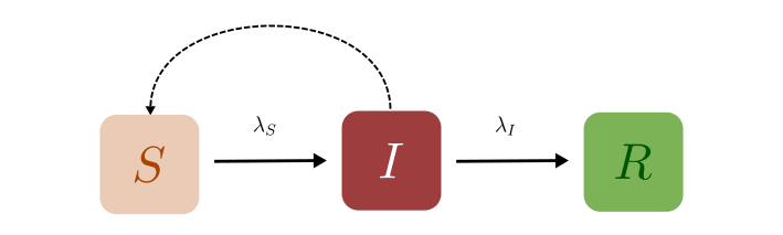
Compartments of the SIR model
The individuals in the SIR model can be in one of the three compartments at any given time, (S)usceptible, (I)nfected, or (R)ecovered. Infected individuals can “infect” the Susceptible, causing them to transition to the Infected compartment, from which they will eventually recover. In what follows we will use the letters S, I, and R to represent both the individual compartments as well as the numbers in each of these compartments. The context should make it clear what we are referring to. In addition, we make some assumptions:
Susceptible individuals can only leave this compartment if they have been infected, and the total number of individuals in the population is conserved. In other words, we ignore the effects of birth and death rates.
The rate of change of \(S(t)\), the number of susceptibles, depends on the number of individuals currently susceptible, the number currently infected, and a parameter that governs the amount of contact between susceptibles and infected.
We also assume that some fixed fraction (say, \(\gamma\)) of the infected group will recover on any given day. Keep in mind that when we say someone has “Recovered”, what we mean (in this model) is that they are no longer infectious or susceptible to the disease and therefore cannot contribute to its spread.
Mean-field or “Well-mixed” solution to this model
This system is modelled by a set of coupled, nonlinear, first order ordinary differential equations. S, I, R are the variables, while \(\beta\) and \(\gamma\) are the parameters of this model. The terms on the left hand side represent rates of change. In this case, change in population of S,I,R per day.
Exercise
Why is there a negative sign in the equation for \(S(t)\)?
Convince yourself that \(\beta\) represents the average number of contacts per unit time between an infected individual and a susceptible individual.
Show that the total population \(N = S+I+R\) is fixed (i.e. that this is a closed system). This is often a very good check to see if your simulation is running correctly!
By inspecting the equations, you can see that the parameters \(\beta\) and \(\gamma\) differ in nature. \(\gamma\) is just the fraction of infected individuals recovering per day. \(\beta\), on the other hand, is a way of quantifying assumption no. 2 from earlier. We want to express that the probability of infection depends on the contact between the infected and the susceptible. This amount of contact is determined by multiplying S and I. We call \(\beta\) the transmission coefficient.
Each infected individual meets a fraction of the total number of susceptibles and infects them at some “transmission rate”. The “contact probability” decides how the transmission scales with the population. Two specific types of scaling can be chosen, depending on the type of disease.
Contact probability = 1. In this case, we assume that infected individuals meet all the susceptibles in one day. Therefore, the larger the population, the faster the spread of disease. This can be used to model a large number of people crowded in an enclosed space. Such a scaling is often appropriate in the case of plant and animal diseases. This is known as density dependent scaling.
Contact probability = \(\mathbf{1/N}\). In this case, we assume the infected individual meets a constant number of people (say \(\lambda_S\)) every day. Of these, the fraction of susceptibles is \(S/N\). This assumption holds for most human diseases, where contact is determined by social factors. This is known as frequency dependent scaling.
The distinction between these two types of scaling only occurs when the total population size is not fixed, since otherwise the factor of \(N\) could simply be absorbed into the definition of \(\beta\). In what follows, we will be using frequency dependent scaling. As a result, Equation (\ref{1}) above can be rewritten as:
Exercise
Show that, because of the extra factor of \(N\), the solutions to this differential equation will be independent of \(N\). (Hint: Rewrite the equations in terms of \(s(t) = S(t)/N\), \(i(t) = I(t)/N\), and \(r(t) = R(t)/N\).)
It turns out that finding the exact solution to this equation as a function of time is not possible. However, an implicit solution can be found. By dividing the first and third equations, show that
\[s(t) = s(0)\,e^{-R_0 r(t)},\]where the quantity \(R_0\) is called the reproductive ratio. Show that \(R_0\) is independent of \(N\).
Now, repeat the previous question for the system denoted by Equation (\ref{1}). Show that in that case, \(R_0\) depends on the total population \(N\).
The above differential equations represented in Equation (\ref{2}) can be easily solved numerically to obtain the curves for \(S\), \(I\), and \(R\) shown in the figure below.
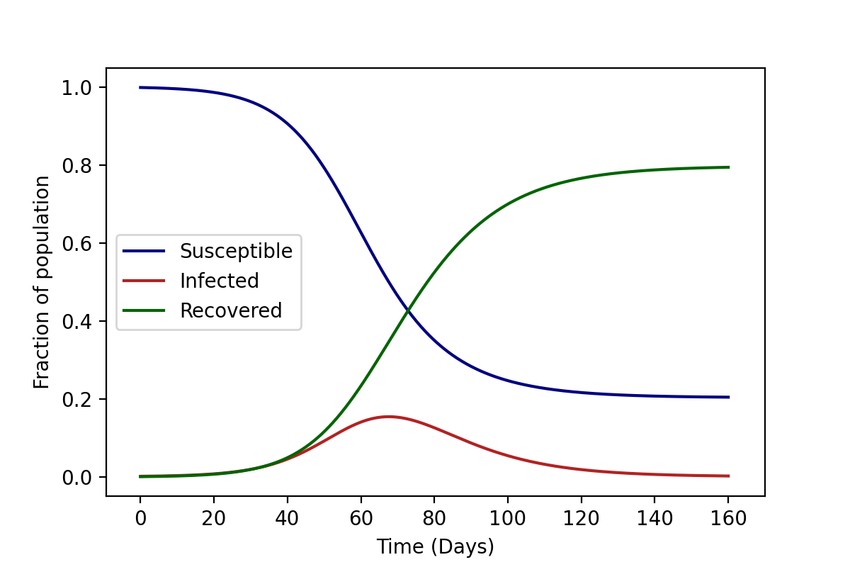
Of course, these solutions are deterministic. This is because we assume the transition rates between the compartments are fixed, the population is well-mixed and we treat all individuals as identical.
Note
A well-mixed population is one in which any infected individual has a probability of contacting any susceptible individual that can be approximated reasonably well by the average probability of susceptible-infected interaction. This is often the most problematic assumption, but is easily relaxed in more complex models.
Stochastic solutions to this model
What happens when the population doesn’t behave in a “well-mixed” manner? For example, consider a population where individuals move between their homes and work-places. In this case, all individuals might not have the same number of contacts. Some individuals might work in high-density workplaces and come in contact with many more individuals and spread the disease at a faster rate than others. The well-mixed scenario also assumes that everyone in a population is identical. We might want to account for the heterogeneity of individuals in the population: some agents might intrinsically be more likely to get infected than others. And lastly we might also want to implement different interventions like a lockdown where only certain agents are allowed to move, and not others.
For all of the above cases, the well-mixed system is inadequate since it assumes that all individuals are identical and indistinguishable. To get around these limitations, one approach is to treat each individual as a separate agent with attributes. These heterogeneous agents interact with each other, spreading the infection. However, keeping track of individual agents is computationally very resource-intensive, even if the questions we can answer are broader.
One of the most well-known methods to implement such simulations is the Gillespie Algorithm. Our framework uses a much simpler discrete time approximation of this method. (The steps for this algorithm are outlined in the box below.) We first consider that all the individuals are in a single location, i.e. everyone is in contact with everyone else. However, in the next section, we will relax this assumption and allow for networks of individuals to be formed. The basic idea is as follows:
Algorithm
Divide the total time into steps of $\Delta t$, and at every time-step we loop over all agents.
If the agent is susceptible, we compute the number of infected individuals who could potentially infect them (”$I$”). Then, with some probability $$p_\text{SI} = \lambda_S\frac{I}{N}\Delta t,$$ we transition them to the infected compartment.
If the agent is already infected, we transition them to the recovered compartment with a probability $$p_\text{IR} = \lambda_I\,\Delta t.$$
If they have recovered, do nothing.
Repeat the entire process until there are no more infected individuals, or the total time has elapsed.
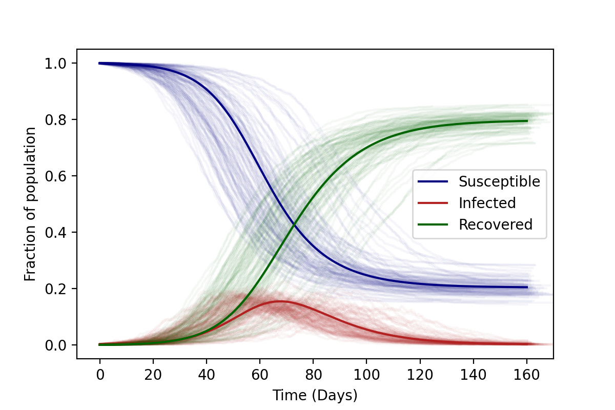
The results of such a stochastic simulation are shown in the figure below. Each faintly visible curve represents a realisation of the stochastic algorithm starting from the same initial conditions. As you can see, the progress of the disease is no longer deterministic. However (in case all agents are in a single location), the average over all of these stochastic runs results in the “well-mixed” solutions (boldly visible curves). Comparing the average of several stochastic runs to the deterministic solution is one way to check your code.